An Introduction to Symbolic Music Processing with Partitura

Partitura is python 3 package for symbolic music processing developed and maintained at OFAI Vienna / CP JKU Linz (and other contributors). It’s inteded to give a lightweight musical part representation that makes many score properties easily accessible for a variety of tasks. Furthermore it’s a very useful I/O utility to parse computer formats of symbolic music.

1. Install and import

Partitura is available in github https://github.com/CPJKU/partitura

You can install it with pip install partitura.

However if you are interested in features that still have to be officially released, it’s better to install the develop branch.

# Install partitura
! pip install partitura

# To be able to access helper modules in the repo for this tutorial
# (not necessary if the jupyter notebook is run locally instead of google colab)
!git clone https://github.com/CPJKU/partitura_tutorial.git
import warnings
warnings.filterwarnings('ignore')
import sys, os
sys.path.insert(0, os.path.join(os.getcwd(), "partitura_tutorial", "content"))
sys.path.insert(0,'/content/partitura_tutorial/content')

import glob
import partitura as pt
import numpy as np
import matplotlib.pyplot as plt

Dataset for this tutorial

In this tutorial we are going to use the Vienna 4x22 Corpus which consists of performances of 4 classical piano pieces, which have been aligned to their corresponding scores.

The dataset contains:

• Scores in MusicXML format (4 scores)

• Performances in MIDI files (88 in total, 22 performances per piece, each by a different pianist)

• Score to performance alignments in Match file format (88 in total one file per performance)

# setup the dataset
from load_data import init_dataset
DATASET_DIR = init_dataset()
MUSICXML_DIR = os.path.join(DATASET_DIR, 'musicxml')
MIDI_DIR = os.path.join(DATASET_DIR, 'midi')
MATCH_DIR = os.path.join(DATASET_DIR, 'match')

2. Loading and Exporting Files

One of the main use cases of partitura is to load and export common symbolic music formats.

Reading

Symbolic Scores

These methods return a Part, a PartGroup or a list of Part objects.

Format	Method	Notes
MusicXML	partitura.load_musicxml
MIDI	partitura.load_score_midi	Pitch spelling, key signature (optional) and other information is inferred with methods in partitura.musicanalysis.
MEI	partitura.load_mei
Humdrum Kern	partitura.load_kern
MuseScore	partitura.load_via_musescore	Requires MuseScore. Loads all formats supported by MuseScore. Support on Windows is still untested.

Symbolic Performances

These methods return a PerformedPart.

Format	Method	Notes
MIDI	partitura.load_performance_midi	Loads MIDI file as a performance, including track, channel and program information. Time signature and tempo information are only used to compute the time of the MIDI messages in seconds. Key signature information is ignored

Alignments

These methods return score-to-performance alignment (discussed below).

Format	Method	Notes
Match file	partitura.load_match	Returns alignment, a performance as PerformedPart and optionally a Part. See usage below.
Nakamura et al. corresp file	partitura.load_nakamuracorresp
Nakamura et al. match file	partitura.load_nakamuramatch

Writing

Symbolic Scores

Support for MEI and Humdrum Kern is coming!

Format	Method	Notes
MusicXML	partitura.save_musicxml
MIDI	partitura.save_score_midi	Includes Key signature, time signature and tempo information.

Symbolic Performances

Format	Method	Notes
MIDI	partitura.save_performance_midi	Does not include key signature or time signature information

Alignments

A companion library for music alignment is in preparation!

Format	Method	Notes
Match file	partitura.save_match

3. Internal Representations

The part object is the central object of partitura. It contains a score. - it is a timeline object - time is measured in divs - its elements are timed objects, i.e. they have a starting time and an ending time - external score files are loaded into a part - parts can be exported into score files - it contains many useful methods related to its properties

Here’s a visual representation of the part object representing the first measure of Chopin’s Nocturne Op. 9 No. 2

path_to_musicxml = pt.EXAMPLE_MUSICXML
part = pt.load_musicxml(path_to_musicxml)[0]
print(part.pretty())

Part id="P1" name="Piano"
 │
 ├─ TimePoint t=0 quarter=12
 │   │
 │   └─ starting objects
 │       │
 │       ├─ 0--48 Measure number=1
 │       ├─ 0--48 Note id=n01 voice=1 staff=2 type=whole pitch=A4
 │       ├─ 0--48 Page number=1
 │       ├─ 0--24 Rest id=r01 voice=2 staff=1 type=half
 │       ├─ 0--48 System number=1
 │       └─ 0-- TimeSignature 4/4
 │
 ├─ TimePoint t=24 quarter=12
 │   │
 │   ├─ ending objects
 │   │   │
 │   │   └─ 0--24 Rest id=r01 voice=2 staff=1 type=half
 │   │
 │   └─ starting objects
 │       │
 │       ├─ 24--48 Note id=n02 voice=2 staff=1 type=half pitch=C5
 │       └─ 24--48 Note id=n03 voice=2 staff=1 type=half pitch=E5
 │
 └─ TimePoint t=48 quarter=12
     │
     └─ ending objects
         │
         ├─ 0--48 Measure number=1
         ├─ 0--48 Note id=n01 voice=1 staff=2 type=whole pitch=A4
         ├─ 24--48 Note id=n02 voice=2 staff=1 type=half pitch=C5
         ├─ 24--48 Note id=n03 voice=2 staff=1 type=half pitch=E5
         ├─ 0--48 Page number=1
         └─ 0--48 System number=1

Each part object contains a list notes. Notes inherit from the TimedObject class. Like all TimedObjects they contain a (possibly coincident) start time and end time, encoded as TimePoint objects.

part.notes

[<partitura.score.Note at 0x7fb004c3bc70>,
 <partitura.score.Note at 0x7fb0048fb790>,
 <partitura.score.Note at 0x7fb0048fb7f0>]

dir(part.notes[0])

['__class__',
 '__delattr__',
 '__dict__',
 '__dir__',
 '__doc__',
 '__eq__',
 '__format__',
 '__ge__',
 '__getattribute__',
 '__gt__',
 '__hash__',
 '__init__',
 '__init_subclass__',
 '__le__',
 '__lt__',
 '__module__',
 '__ne__',
 '__new__',
 '__reduce__',
 '__reduce_ex__',
 '__repr__',
 '__setattr__',
 '__sizeof__',
 '__str__',
 '__subclasshook__',
 '__weakref__',
 '_ref_attrs',
 '_sym_dur',
 'alter',
 'alter_sign',
 'articulations',
 'beam',
 'doc_order',
 'duration',
 'duration_from_symbolic',
 'duration_tied',
 'end',
 'end_tied',
 'fermata',
 'id',
 'iter_chord',
 'midi_pitch',
 'octave',
 'ornaments',
 'replace_refs',
 'slur_starts',
 'slur_stops',
 'staff',
 'start',
 'step',
 'symbolic_duration',
 'tie_next',
 'tie_next_notes',
 'tie_prev',
 'tie_prev_notes',
 'tuplet_starts',
 'tuplet_stops',
 'voice']

You can create notes (without timing information) and then add it to a part by specifying start and end times (in divs!). Use each note object only once! You can remove notes from a part.

a_new_note = pt.score.Note(id='n04', step='A', octave=4, voice=1)
part.add(a_new_note, start=3, end=15)
# print(part.pretty())

part.remove(a_new_note)
# print(part.pretty())

Integer divs are useful for encoding scores but unwieldy for human readers. Partitura offers a variety of *unit*_maps from the timeline unit “div” to musical units such as “beats” (in two different readings) or “quarters”. For the inverse operation the corresponding inv_*unit*_map exist as well. Quarter to div ratio is a fixed value for a part object, but units like beats might change with time signature, so these maps are implemented as part methods.

Let’s look at how to get the ending position in beats of the last note in our example part.

part.beat_map(part.notes[0].end.t)

array(4.)

Some musical information such as key and time signature is valid for a segment of the score but only encoded in one location. To retrieve the “currently active” time or key signature at any score position, maps are available too.

part.time_signature_map(part.notes[0].end.t)

array([4., 4., 4.])

The part class contains a central method iter_all to iterate over all instances of the TimedObject class or its subclasses of a part. The iter_all method returns an iterator and takes five optional parameters: - A TimedObject subclass whose instances are returned. You can find them all in the partitura/partitura/score.py file. Default is all classes. - A include_subclasses flag. If true, instances of subclasses are returned too. E.g. part.iter_all(pt.score.TimedObject, include_subclasses=True) returns all objects or part.iter_all(pt.score.GenericNote, include_subclasses=True) returns all notes (grace notes, standard notes) - A start time in divs to specify the search interval (default is beginning of the part) - An end time in divs to specify the search interval (default is end of the part) - A mode parameter to define whether to search for starting or ending objects, defaults to starting.

for measure in part.iter_all(pt.score.Measure):
    print(measure)

0--48 Measure number=1

for note in part.iter_all(pt.score.GenericNote, include_subclasses=True, start=0, end=24):
    print(note)

0--48 Note id=n01 voice=1 staff=2 type=whole pitch=A4
0--24 Rest id=r01 voice=2 staff=1 type=half

Let’s use class retrieval, time mapping, and object creation together and add a new measure with a single beat-length note at its downbeat. This code works even if you know nothing about the underlying score.

# figure out the last measure position, time signature and beat length in divs
measures = [m for m in part.iter_all(pt.score.Measure)]
last_measure_number = measures[-1].number
append_measure_start =  measures[-1].end.t
Last_measure_ts = part.time_signature_map(append_measure_start)

Last_measure_ts = part.time_signature_map(append_measure_start)
one_beat_in_divs_at_the_end = append_measure_start - part.inv_beat_map(part.beat_map(append_measure_start)-1)
append_measure_end = append_measure_start +  one_beat_in_divs_at_the_end*Last_measure_ts[0]

# add a measure
a_new_measure = pt.score.Measure(number = last_measure_number+1)
part.add(a_new_measure, start=append_measure_start, end=append_measure_end)
# add a note
a_new_note = pt.score.Note(id='n04', step='A', octave=4, voice=1)
part.add(a_new_note, start=append_measure_start, end=append_measure_start+one_beat_in_divs_at_the_end)

# print(part.pretty())

The PerformedPart class is a wrapper for MIDI files. Its structure is much simpler: - a notes property that consists of list of MIDI notes as dictionaries - a controls property that consists of list of MIDI CC messages - some more utility methods and properties

path_to_midifile = pt.EXAMPLE_MIDI
performedpart = pt.load_performance_midi(path_to_midifile)[0]

performedpart.notes

[{'midi_pitch': 69,
  'note_on': 0.0,
  'note_off': 2.0,
  'track': 0,
  'channel': 1,
  'velocity': 64,
  'id': 'n0',
  'sound_off': 2.0},
 {'midi_pitch': 72,
  'note_on': 1.0,
  'note_off': 2.0,
  'track': 0,
  'channel': 2,
  'velocity': 64,
  'id': 'n1',
  'sound_off': 2.0},
 {'midi_pitch': 76,
  'note_on': 1.0,
  'note_off': 2.0,
  'track': 0,
  'channel': 2,
  'velocity': 64,
  'id': 'n2',
  'sound_off': 2.0}]

import numpy as np

def addnote(midipitch, part, voice, start, end, idx):
    """
    adds a single note by midipitch to a part
    """
    offset = midipitch%12
    octave = int(midipitch-offset)/12
    name = [("C",0),
            ("C",1),
            ("D",0),
            ("D",1),
            ("E",0),
            ("F",0),
            ("F",1),
            ("G",0),
            ("G",1),
            ("A",0),
            ("A",1),
            ("B",0)]
    # print( id, start, end, offset)
    step, alter = name[int(offset)]
    part.add(pt.score.Note(id='n{}'.format(idx), step=step,
                        octave=int(octave), alter=alter, voice=voice, staff=str((voice-1)%2+1)),
                        start=start, end=end)

l = 200
p = pt.score.Part('CoK', 'Cat on Keyboard', quarter_duration=8)
dur = np.random.randint(1,20, size=(4,l+1))
ons = np.cumsum(dur, axis = 1)
pitch = np.row_stack((np.random.randint(20,40, size=(1,l+1)),
                      np.random.randint(60,80, size=(1,l+1)),
                      np.random.randint(40,60, size=(1,l+1)),
                      np.random.randint(40,60, size=(1,l+1))
                     ))

for k in range(l):
    for j in range(4):
        addnote(pitch[j,k], p, j+1, ons[j,k], ons[j,k]+dur[j,k+1], "v"+str(j)+"n"+str(k))

p.add(pt.score.TimeSignature(4, 4), start=0)
p.add(pt.score.Clef(1, "G", line = 3, octave_change=0),start=0)
p.add(pt.score.Clef(2, "G", line = 3, octave_change=0),start=0)
pt.score.add_measures(p)
pt.score.tie_notes(p)

# pt.save_score_midi(p, "CatPerformance.mid", part_voice_assign_mode=2)

# pt.save_musicxml(p, "CatScore.xml")

4. Extracting Information from Scores and Performances

For many MIR tasks we need to extract specific information out of scores or performances. Two of the most common representations are note arrays and piano rolls.

Note that there is some overlap in the way that these terms are used.

Partitura provides convenience methods to extract these common features in a few lines!

A note array is a 2D array in which each row represents a note in the score/performance and each column represents different attributes of the note.

In partitura, note arrays are structured numpy arrays, which are ndarrays in which each “column” has a name, and can be of different datatypes. This allows us to hold information that can be represented as integers (MIDI pitch/velocity), floating point numbers (e.g., onset time) or strings (e.g., note ids).

In this tutorial we are going to cover 3 main cases

• Getting a note array from Part and PerformedPart objects

• Extra information and alternative ways to generate a note array

• Creating a custom note array from scratch from a Part object

4.1.1. Getting a note array from Part and PerformedPart objects

Getting a note array from Part objects

# Note array from a score

# Path to the MusicXML file
score_fn = os.path.join(MUSICXML_DIR, 'Chopin_op38.musicxml')

# Load the score into a `Part` object
score_part = pt.load_musicxml(score_fn)

# Get note array.
score_note_array = score_part.note_array()

It is that easy!

# Lets see the first notes in this note array
print(score_note_array[:10])

[(-4., 1., -2. , 0.5,  0,  8, 60, 4, 'n2', 16)
 (-4., 1., -2. , 0.5,  0,  8, 72, 1, 'n1', 16)
 (-3., 2., -1.5, 1. ,  8, 16, 60, 4, 'n4', 16)
 (-3., 2., -1.5, 1. ,  8, 16, 72, 1, 'n3', 16)
 (-1., 1., -0.5, 0.5, 24,  8, 60, 4, 'n6', 16)
 (-1., 1., -0.5, 0.5, 24,  8, 72, 1, 'n5', 16)
 ( 0., 2.,  0. , 1. , 32, 16, 60, 4, 'n8', 16)
 ( 0., 2.,  0. , 1. , 32, 16, 72, 1, 'n7', 16)
 ( 2., 1.,  1. , 0.5, 48,  8, 60, 4, 'n10', 16)
 ( 2., 1.,  1. , 0.5, 48,  8, 72, 1, 'n9', 16)]

By default, Partitura includes some of the most common note-level information in the note array:

print(score_note_array.dtype.names)

('onset_beat', 'duration_beat', 'onset_quarter', 'duration_quarter', 'onset_div', 'duration_div', 'pitch', 'voice', 'id', 'divs_pq')

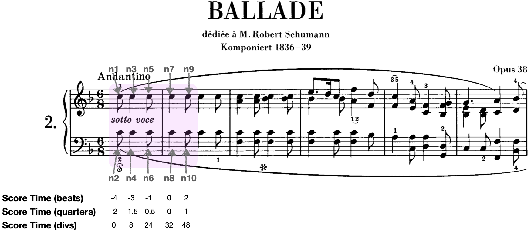
• onset_beat is the onset time in beats (as indicated by the time signature). In partitura, negative onset times in beats represent pickup measures. Onset time 0 is the start of the first measure.

• duration_beat is the duration of the note in beats

• onset_quarter is the onset time of the note in quarters (independent of the time signature). Similarly to onset time in beats, negative onset times in quarters represent pickup measures and onset time 0 is the start of the first measure.

• duration_quarteris the duration of the note in quarters

• onset_div is the onset of the note in divs, which is generally a number that allows to represent the note position and duration losslessly with integers. In contrast to onset time in beats or quarters, onset time in divs always start at 0 at the first “element” in the score (which might not necessarily be a note).

• duration_div is the duration of the note in divs.

• pitch is the MIDI pitch (MIDI note number) of the note

• voice is the voice of the note (in polyphonic music, where there can be multiple notes at the same time)

• id is the note id (as appears in MusicXML or MEI formats)

Getting a note array from a PerformedPart

In a similar way, we can obtain a note array from a MIDI file in a few lines

# Note array from a performance

# Path to the MIDI file
performance_fn = os.path.join(MIDI_DIR, 'Chopin_op38_p01.mid')

# Loading the file to a PerformedPart
performance_part = pt.load_performance_midi(performance_fn)

# Get note array!
performance_note_array = performance_part.note_array()

Since performances contain have other information not included in scores, the default fields in the note array are a little bit different:

print(performance_note_array.dtype.names)

('onset_sec', 'duration_sec', 'pitch', 'velocity', 'track', 'channel', 'id')

• onset_sec is the onset time of the note in seconds. Onset time in seconds is always \(\geq 0\) (otherwise, the performance would violate the laws of physics ;)

• duration_sec is the duration of the note in seconds

• pitch is the MIDI pitch

• velocity is the MIDI velocity

• track is the track number in the MIDI file

• channel is the channel in the MIDI file

• id is the ID of the notes (automatically generated for MIDI file according to onset time)

print(performance_note_array[:5])

[(5.6075 , 5.5025 , 72, 37, 0, 0, 'n0')
 (5.63375, 5.47625, 60, 27, 0, 0, 'n1')
 (6.07   , 5.04   , 72, 45, 0, 0, 'n2')
 (6.11125, 4.99875, 60, 26, 0, 0, 'n3')
 (6.82625, 4.28375, 60, 39, 0, 0, 'n4')]

We can also create a PerformedPart directly from a note array

note_array = np.array(
    [(60, 0, 2, 40),
     (65, 0, 1, 15),
     (67, 0, 1, 72),
     (69, 1, 1, 90),
     (66, 2, 1, 80)],
    dtype=[("pitch", "i4"),
           ("onset_sec", "f4"),
           ("duration_sec", "f4"),
           ("velocity", "i4"),
          ]
)

# Note array to `PerformedPart`
performed_part = pt.performance.PerformedPart.from_note_array(note_array)

We can then export the PerformedPart to a MIDI file!

# export as MIDI file
pt.save_performance_midi(performed_part, "example.mid")

4.1.2. Extra information and alternative ways to generate a note array

Sometimes we require more information in a note array.

extended_score_note_array = pt.utils.music.ensure_notearray(
    score_part,
    include_pitch_spelling=True, # adds 3 fields: step, alter, octave
    include_key_signature=True, # adds 2 fields: ks_fifths, ks_mode
    include_time_signature=True, # adds 2 fields: ts_beats, ts_beat_type
    # include_metrical_position=True, # adds 3 fields: is_downbeat, rel_onset_div, tot_measure_div
    include_grace_notes=True # adds 2 fields: is_grace, grace_type
)

extended_score_note_array.dtype.names

('onset_beat',
 'duration_beat',
 'onset_quarter',
 'duration_quarter',
 'onset_div',
 'duration_div',
 'pitch',
 'voice',
 'id',
 'step',
 'alter',
 'octave',
 'is_grace',
 'grace_type',
 'ks_fifths',
 'ks_mode',
 'ts_beats',
 'ts_beat_type',
 'ts_mus_beats',
 'divs_pq')

print(extended_score_note_array[['id',
                                 'step',
                                 'alter',
                                 'octave',
                                 'ks_fifths',
                                 'ks_mode', #'is_downbeat'
                                 ]][:10])

[('n2', 'C', 0, 4, -1, 1) ('n1', 'C', 0, 5, -1, 1)
 ('n4', 'C', 0, 4, -1, 1) ('n3', 'C', 0, 5, -1, 1)
 ('n6', 'C', 0, 4, -1, 1) ('n5', 'C', 0, 5, -1, 1)
 ('n8', 'C', 0, 4, -1, 1) ('n7', 'C', 0, 5, -1, 1)
 ('n10', 'C', 0, 4, -1, 1) ('n9', 'C', 0, 5, -1, 1)]

4.1.3. Creating a custom note array from scratch from a Part object

Sometimes we are interested in other note-level information that is not included in the standard note arrays. With partitura we can create such a note array easily!

For example, imagine that we want a note array that includes whether the notes have an accent mark.

# Path to the MusicXML file
score_fn = os.path.join(MUSICXML_DIR, 'Chopin_op10_no3.musicxml')

# Load the score into a `Part` object
score_part = pt.load_musicxml(score_fn)[0]

def get_accent_note_array(part):

    fields = [("onset_beat", "f4"),
              ("pitch", "i4"),
              ("accent", "i4")]
    # Get all notes in the part
    notes = part.notes_tied
    # Beat map (maps divs to score time in beats)
    beat_map = part.beat_map
    N = len(notes)
    note_array = np.zeros(N, dtype=fields)
    for i, n in enumerate(notes):
        # MIDI pitch
        note_array[i]['pitch'] = n.midi_pitch
        # Get the onset time in beats
        note_array[i]['onset_beat'] = beat_map(n.start.t)

        # Iterate over articulations in the note
        if n.articulations:
            for art in n.articulations:
                if art == 'accent':
                    note_array[i]['accent'] = 1
    return note_array

accent_note_array = get_accent_note_array(score_part)

accented_note_idxs = np.where(accent_note_array['accent'])
print(accent_note_array[accented_note_idxs][:5])

[(0.25, 47, 1) (1.25, 47, 1) (2.25, 47, 1) (3.  , 68, 1) (3.25, 47, 1)]

Piano rolls are 2D matrices that represent pitch and time information. The time represents time steps (at a given resolution), while the pitch axis represents which notes are active at a given time step. We can think of piano rolls as the symbolic equivalent of spectrograms.

Extracting a piano roll

# TODO: change the example
# Path to the MusicXML file
score_fn = os.path.join(MUSICXML_DIR, 'Chopin_op10_no3.musicxml')

# Load the score
score_part = pt.load_musicxml(score_fn)
# compute piano roll
pianoroll = pt.utils.compute_pianoroll(score_part)

The compute_pianoroll method has a few arguments to customize the resulting piano roll

piano_range = True
time_unit = 'beat'
time_div = 10
pianoroll = pt.utils.compute_pianoroll(
    note_info=score_part, # a `Part`, `PerformedPart` or a note array
    time_unit=time_unit, # beat, quarter, div, sec, etc. (depending on note_info)
    time_div=time_div, # Number of cells per time unit
    piano_range=piano_range # Use range of the piano (88 keys)
)

An important thing to remember is that in piano rolls generated by compute_pianoroll, rows (the vertical axis) represent the pitch dimension and the columns (horizontal) the time dimension. This results in a more intuitive way of plotting the piano roll. For other applications the transposed version of this piano roll might be more useful (i.e., rows representing time steps and columns representing pitch information).

Since piano rolls can result in very large matrices where most of the elements are 0, the output of compute_pianoroll is a scipy sparse matrix. To convert it to a regular numpy array, we can simply use pianoroll.toarray()

Let’s plot the piano roll!

fig, ax = plt.subplots(1, figsize=(20, 10))
ax.imshow(pianoroll.toarray(), origin="lower", cmap='gray', interpolation='nearest', aspect='auto')
ax.set_xlabel(f'Time ({time_unit}s/{time_div})')
ax.set_ylabel('Piano key' if piano_range else 'MIDI pitch')
plt.show()

In some cases, we want to know the “coordinates” of each of the notes in the piano roll. The compute_pianoroll method includes an option to return

pianoroll, note_indices = pt.utils.compute_pianoroll(score_part, return_idxs=True)

# MIDI pitch, start, end
print(note_indices[:5])

[[59  0  4]
 [40  4 12]
 [40  4  6]
 [56  4  6]
 [64  4  8]]

Generating a note array from a piano roll

Partitura also includes a method to generate a note array from a piano roll, which can be used to generate a MIDI file. This method would be useful, e.g., for music generation tasks

pianoroll = pt.utils.compute_pianoroll(score_part)

new_note_array = pt.utils.pianoroll_to_notearray(pianoroll)

# We can export the note array to a MIDI file
ppart = pt.performance.PerformedPart.from_note_array(new_note_array)

pt.save_performance_midi(ppart, "newmidi.mid")

5. Handling Alignment Information (Match files)

An important use case of partitura is to handle symbolic alignment information

Note that partitura itself does not contain methods for alignment

Partitura supports 2 formats for encoding score-to-performance alignments

• Our match file format, introduced by Gerhard et al. ;)

  • Datasets including match files: Vienna4x22, Magaloff, Zeilinger, Batik, and soon ASAP!

• The format introduced by Nakamura et al. (2017)

Let’s load an alignment!

We have two common use cases

• We have both the match file and the symbolic score file (e.g., MusicXML or MEI)

• We have only the match file (only works for our format!)

5.1.1. Loading an alignment if we only have a match file

A useful property of match files is that they include information about the score and the performance. Therefore, it is possible to create both a Part and a PerformedPart directly from a match file.

• Match files contain all information included in performances in MIDI files, i.e., a MIDI file could be reconstructed from a match file.

• Match files include all information information about pitch spelling and score position and duration of the notes in the score, as well as time and key signature information, and can encode some note-level markings, like accents. Nevertheless, it is important to note that the score information included in a match file is not necessarily complete. For example, match files do not generally include dynamics or tempo markings.

# path to the match
match_fn = os.path.join(MATCH_DIR, 'Chopin_op10_no3_p01.match')
# loading a match file
performed_part, alignment, score_part = pt.load_match(match_fn, create_part=True)

5.1.2. Loading an alignment if we have both score and match files

In many cases, however, we have access to both the score and match files. Using the original score file has a few advantages:

• It ensures that the score information is correct. Generating a Part from a match file involves inferring information for non-note elements (e.g., start and end time of the measures, voice information, clefs, staves, etc.).

• If we want to load several performances of the same piece, we can load the score only once!

This should be the preferred way to get alignment information!

# path to the match
match_fn = os.path.join(MATCH_DIR, 'Chopin_op10_no3_p01.match')
# Path to the MusicXML file
score_fn = os.path.join(MUSICXML_DIR, 'Chopin_op10_no3.musicxml')
# Load the score into a `Part` object
score_part = pt.load_musicxml(score_fn)[0]

# loading a match file
performed_part, alignment = pt.load_match(match_fn)

Score-to-performance alignments are represented by lists of dictionaries, which contain the following keys:

• label

  • 'match': there is a performed note corresponding to a score note

  • 'insertion': the performed note does not correspond to any note in the score

  • 'deletion': there is no performed note corresponding to a note in the score

  • 'ornament': the performed note corresponds to the performance of an ornament (e.g., a trill). These notes are matched to the main note in the score. Not all alignments (in the datasets that we have) include ornamnets! Otherwise, ornaments are just treated as insertions.

• score_id: id of the note in the score (in the Part object) (only relevant for matches, deletions and ornaments)

• performance_id: Id of the note in the performance (in the PerformedPart) (only relevant for matches, insertions and ornaments)

alignment[:10]

[{'label': 'match', 'score_id': 'n1', 'performance_id': 0},
 {'label': 'match', 'score_id': 'n2', 'performance_id': 2},
 {'label': 'match', 'score_id': 'n3', 'performance_id': 3},
 {'label': 'match', 'score_id': 'n4', 'performance_id': 1},
 {'label': 'match', 'score_id': 'n5', 'performance_id': 5},
 {'label': 'match', 'score_id': 'n6', 'performance_id': 4},
 {'label': 'match', 'score_id': 'n7', 'performance_id': 6},
 {'label': 'match', 'score_id': 'n8', 'performance_id': 7},
 {'label': 'match', 'score_id': 'n9', 'performance_id': 8},
 {'label': 'match', 'score_id': 'n10', 'performance_id': 9}]

Partitura includes a few methods for getting information from the alignments.

Let’s start by getting the subset of score notes that have a corresponding performed note

# note array of the score
snote_array = score_part.note_array()
# note array of the performance
pnote_array = performed_part.note_array()
# indices of the notes that have been matched
matched_note_idxs = pt.utils.music.get_matched_notes(snote_array, pnote_array, alignment)

# note array of the matched score notes
matched_snote_array = snote_array[matched_note_idxs[:, 0]]
# note array of the matched performed notes
matched_pnote_array = pnote_array[matched_note_idxs[:, 1]]

Comparing tempo curves

In this example, we are going to compare tempo curves of different performances of the same piece. Partitura includes a utility function called get_time_maps_from_alignmentwhich creates functions (instances of `scipy.interpolate.interp1d <https://docs.scipy.org/doc/scipy/reference/generated/scipy.interpolate.interp1d.html>`__) that map score time to performance time (and the other way around).

# get all match files
matchfiles = glob.glob(os.path.join(MATCH_DIR, 'Chopin_op10_no3_p*.match'))
matchfiles.sort()

# Score time from the first to the last onset
score_time = np.linspace(snote_array['onset_beat'].min(),
                         snote_array['onset_beat'].max(),
                         100)
# Include the last offset
score_time_ending = np.r_[
    score_time,
    (snote_array['onset_beat'] + snote_array['duration_beat']).max() # last offset
]

tempo_curves = np.zeros((len(matchfiles), len(score_time)))
for i, matchfile in enumerate(matchfiles):
    # load alignment
    performance, alignment = pt.load_match(matchfile)
    ppart = performance[0]
    # Get score time to performance time map
    _, stime_to_ptime_map = pt.utils.music.get_time_maps_from_alignment(
        ppart, score_part, alignment)
    # Compute naïve tempo curve
    performance_time = stime_to_ptime_map(score_time_ending)
    tempo_curves[i,:] = 60 * np.diff(score_time_ending) / np.diff(performance_time)

fig, ax = plt.subplots(1, figsize=(15, 8))
color = plt.cm.rainbow(np.linspace(0, 1, len(tempo_curves)))
for i, tempo_curve in enumerate(tempo_curves):
    ax.plot(score_time, tempo_curve,
            label=f'pianist {i + 1:02d}', alpha=0.4, c=color[i])

# plot average performance
ax.plot(score_time, tempo_curves.mean(0), label='average', c='black', linewidth=2)

# get starting time of each measure in the score
measure_times = score_part.beat_map([measure.start.t for measure in score_part.iter_all(pt.score.Measure)])
# do not include pickup measure
measure_times = measure_times[measure_times >= 0]
ax.set_title('Chopin Op. 10 No. 3')
ax.set_xlabel('Score time (beats)')
ax.set_ylabel('Tempo (bpm)')
ax.set_xticks(measure_times)
plt.legend(frameon=False, bbox_to_anchor = (1.15, .9))
plt.grid(axis='x')
plt.show()

The end of the tutorial, the start of your yet untold adventures in symbolic music processing…

Thank you for trying out partitura! We hope it serves you well.

If you miss a particular functionality or encounter a bug, we appreciate it if you raise an issue on GitHub: https://github.com/CPJKU/partitura/issues